Load Predefined Control System Environments

Reinforcement Learning Toolbox™ software provides several predefined control system environments for which the actions, observations, rewards, and dynamics are already defined. You can use these environments to:

Learn reinforcement learning concepts.
Gain familiarity with Reinforcement Learning Toolbox software features.
Test your own reinforcement learning agents.

You can load the following predefined MATLAB^® control system environments using the rlPredefinedEnv function.

Environment	Agent Task
Cart-pole	Balance a pole on a moving cart by applying forces to the cart using either a discrete or continuous action space.
Double integrator	Control a second-order dynamic system using either a discrete or continuous action space.
Simple pendulum with image observation	Swing up and balance a simple pendulum using either a discrete or continuous action space.

You can also load predefined MATLAB grid world environments. For more information, see Load Predefined Grid World Environments.

Cart-Pole Environments

The goal of the agent in the predefined cart-pole environments is to balance a pole on a moving cart by applying horizontal forces to the cart. The pole is considered successfully balanced if both of the following conditions are satisfied:

The pole angle remains within a given threshold of the vertical position, where the vertical position is zero radians.
The magnitude of the cart position remains below a given threshold.

There are two cart-pole environment variants, which differ by the agent action space.

Discrete — Agent can apply a force of either F_max or -F_max to the cart, where F_max is the MaxForce property of the environment.
Continuous — Agent can apply any force within the range [-F_max,F_max].

To create a cart-pole environment, use the rlPredefinedEnv function.

Discrete action space

env = rlPredefinedEnv('CartPole-Discrete');

Continuous action space

env = rlPredefinedEnv('CartPole-Continuous');

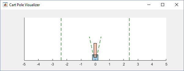
You can visualize the cart-pole environment using the plot function. The plot displays the cart as a blue square and the pole as a red rectangle.

plot(env)

Basic visualization of a cart pole environment, with cart (indicated by a blue square) positioned at the origin, an erected pole (indicated by a pink rectangle) attached on top of the cart, and green lines indicating limits for the cart position and the pole angle.

To visualize the environment during training, call plot before training and keep the visualization figure open.

For examples showing how to train agents in cart-pole environments, see the following:

Environment Properties

Property	Description	Default
`Gravity`	Acceleration due to gravity in meters per second squared	`9.8`
`MassCart`	Mass of the cart in kilograms	`1`
`MassPole`	Mass of the pole in kilograms	`0.1`
`Length`	Half the length of the pole in meters	`0.5`
`MaxForce`	Maximum horizontal force magnitude in newtons	`10`
`Ts`	Sample time in seconds	`0.02`
`ThetaThresholdRadians`	Pole angle threshold in radians	`0.2094`
`XThreshold`	Cart position threshold in meters	`2.4`
`RewardForNotFalling`	Reward for each time step the pole is balanced	`1`
`PenaltyForFalling`	Reward penalty for failing to balance the pole	Discrete — `-5` Continuous — `-50`
`State`	Environment state, specified as a column vector with the following state variables: Cart position Derivative of cart position Pole angle Derivative of pole angle	`[0 0 0 0]'`

Actions

In the cart-pole environments, the agent interacts with the environment using a single action signal, the horizontal force applied to the cart. The environment contains a specification object for this action signal. For the environment with a:

Discrete action space, the specification is an rlFiniteSetSpec object.
Continuous action space, the specification is an rlNumericSpec object.

For more information on obtaining action specifications from an environment, see getActionInfo.

Observations

In the cart-pole system, the agent can observe all the environment state variables in env.State. For each state variable, the environment contains an rlNumericSpec observation specification. All the states are continuous and unbounded.

For more information on obtaining observation specifications from an environment, see getObservationInfo.

Reward

The reward signal for this environment consists of two components.

A positive reward for each time step that the pole is balanced, that is, the cart and pole both remain within their specified threshold ranges. This reward accumulates over the entire training episode. To control the size of this reward, use the RewardForNotFalling property of the environment.
A one-time negative penalty if either the pole or cart moves outside of their threshold range. At this point, the training episode stops. To control the size of this penalty, use the PenaltyForFalling property of the environment.

Double Integrator Environments

The goal of the agent in the predefined double integrator environments is to control the position of a mass in a second-order system by applying a force input. Specifically, the second-order system is a double integrator with a gain.

Training episodes for these environments end when either of the following events occurs:

The mass moves beyond a given threshold from the origin.
The norm of the state vector is less than a given threshold.

There are two double integrator environment variants, which differ by the agent action space.

Discrete — Agent can apply a force of either F_max or -F_max to the cart, where F_max is the MaxForce property of the environment.
Continuous — Agent can apply any force within the range [-F_max,F_max].

To create a double integrator environment, use the rlPredefinedEnv function.

Discrete action space

env = rlPredefinedEnv('DoubleIntegrator-Discrete');

Continuous action space

env = rlPredefinedEnv('DoubleIntegrator-Continuous');

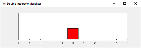
You can visualize the double integrator environment using the plot function. The plot displays the mass as a red rectangle.

plot(env)

Basic visualization of a double integrator environment, with a red square positioned at the origin.

To visualize the environment during training, call plot before training and keep the visualization figure open.

For examples showing how to train agents in double integrator environments, see the following:

Environment Properties

Property	Description	Default
`Gain`	Gain for the double integrator	`1`
`Ts`	Sample time in seconds	`0.1`
`MaxDistance`	Distance magnitude threshold in meters	`5`
`GoalThreshold`	State norm threshold	`0.01`
`Q`	Weight matrix for observation component of reward signal	`[10 0; 0 1]`
`R`	Weight matrix for action component of reward signal	`0.01`
`MaxForce`	Maximum input force in newtons	Discrete: `2` Continuous: `Inf`
`State`	Environment state, specified as a column vector with the following state variables: Mass position Derivative of mass position	`[0 0]'`

Actions

In the double integrator environments, the agent interacts with the environment using a single action signal, the force applied to the mass. The environment contains a specification object for this action signal. For the environment with a:

Discrete action space, the specification is an rlFiniteSetSpec object.
Continuous action space, the specification is an rlNumericSpec object.

For more information on obtaining action specifications from an environment, see getActionInfo.

Observations

In the double integrator system, the agent can observe both of the environment state variables in env.State. For each state variable, the environment contains an rlNumericSpec observation specification. Both states are continuous and unbounded.

For more information on obtaining observation specifications from an environment, see getObservationInfo.

Reward

The reward signal for this environment is the discrete-time equivalent of the following continuous-time reward, which is analogous to the cost function of an LQR controller.

$r e w a r d = - \int (x' Q x + u' R u) d t$

Here:

Q and R are environment properties.
x is the environment state vector.
u is the input force.

This reward is the episodic reward, that is, the cumulative reward across the entire training episode.

Simple Pendulum Environments with Image Observation

This environment is a simple frictionless pendulum that is initially hangs in a downward position. The training goal is to make the pendulum stand upright without falling over using minimal control effort.

There are two simple pendulum environment variants, which differ by the agent action space.

Discrete — Agent can apply a torque of -2, -1, 0, 1, or 2 to the pendulum.
Continuous — Agent can apply any torque within the range [-2,2].

To create a simple pendulum environment, use the rlPredefinedEnv function.

Discrete action space

env = rlPredefinedEnv('SimplePendulumWithImage-Discrete');

Continuous action space

env = rlPredefinedEnv('SimplePendulumWithImage-Continuous');

For examples showing how to train an agent in this environment, see the following:

Environment Properties

Property	Description	Default
`Mass`	Pendulum mass	`1`
`RodLength`	Pendulum length	`1`
`RodInertia`	Pendulum moment of inertia	`0`
`Gravity`	Acceleration due to gravity in meters per second squared	`9.81`
`DampingRatio`	Damping on pendulum motion	`0`
`MaximumTorque`	Maximum input torque in newtons	`2`
`Ts`	Sample time in seconds	`0.05`
`State`	Environment state, specified as a column vector with the following state variables: Pendulum angle Pendulum angular velocity	`[0 0 ]'`
`Q`	Weight matrix for observation component of reward signal	`[1 0;0 0.1]`
`R`	Weight matrix for action component of reward signal	`1e-3`

Actions

In the simple pendulum environments, the agent interacts with the environment using a single action signal, the torque applied at the base of the pendulum. The environment contains a specification object for this action signal. For the environment with a:

Discrete action space, the specification is an rlFiniteSetSpec object.
Continuous action space, the specification is an rlNumericSpec object.

For more information on obtaining action specifications from an environment, see getActionInfo.

Observations

In the simple pendulum environment, the agent receives the following observation signals:

50-by-50 grayscale image of the pendulum position
Derivative of the pendulum angle

For each observation signal, the environment contains an rlNumericSpec observation specification. All the observations are continuous and unbounded.

For more information on obtaining observation specifications from an environment, see getObservationInfo.

Reward

The reward signal for this environment is

$r_{t} = - (θ_{t}^{2} + 0.1 * {\dot{θ}}_{t}^{2} + 0.001 * u_{t - 1}^{2})$

Here:

θ_t is the pendulum angle of displacement from the upright position.
${\dot{θ}}_{t}$ is the derivative of the pendulum angle.
u_t-1 is the control effort from the previous time step.

Related Examples

Train Reinforcement Learning Agents