Load Predefined Simulink Environments

Reinforcement Learning Toolbox™ software provides predefined Simulink^® environments for which the actions, observations, rewards, and dynamics are already defined. You can use these environments to:

Learn reinforcement learning concepts.
Gain familiarity with Reinforcement Learning Toolbox software features.
Test your own reinforcement learning agents.

You can load the following predefined Simulink environments using the rlPredefinedEnv function.

Environment	Agent Task
Simple pendulum Simulink model	Swing up and balance a simple pendulum using either a discrete or continuous action space.
Cart-pole Simscape™ model	Balance a pole on a moving cart by applying forces to the cart using either a discrete or continuous action space.

For predefined Simulink environments, the environment dynamics, observations, and reward signal are defined in a corresponding Simulink model. The rlPredefinedEnv function creates a SimulinkEnvWithAgent object that the train function uses to interact with the Simulink model.

Simple Pendulum Simulink Model

This environment is a simple frictionless pendulum that initially hangs in a downward position. The training goal is to make the pendulum stand upright without falling over using minimal control effort. The model for this environment is defined in the rlSimplePendulumModel Simulink model.

open_system('rlSimplePendulumModel')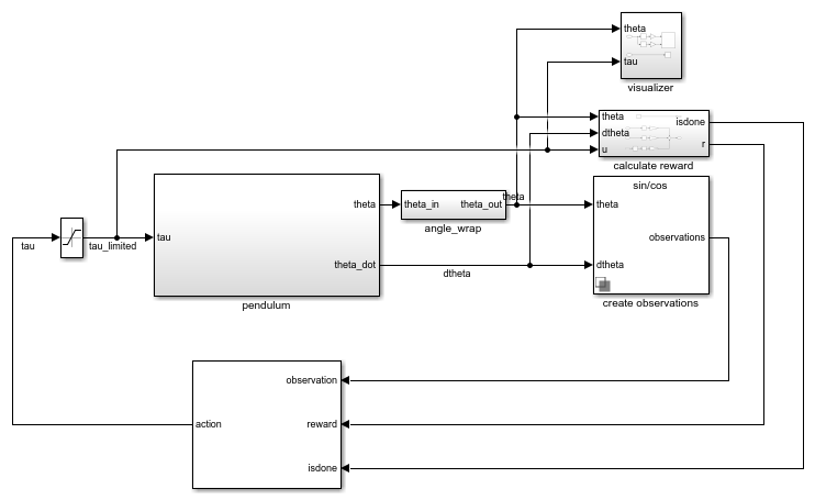

Simulink model of a pendulum system in a feedback loop with an agent block.

There are two simple pendulum environment variants, which differ by the agent action space.

Discrete — Agent can apply a torque of either T_max, 0, or -T_max to the pendulum, where T_max is the max_tau variable in the model workspace.
Continuous — Agent can apply any torque within the range [-T_max,T_max].

To create a simple pendulum environment, use the rlPredefinedEnv function.

Discrete action space

env = rlPredefinedEnv('SimplePendulumModel-Discrete');

Continuous action space

env = rlPredefinedEnv('SimplePendulumModel-Continuous');

For examples that train agents in the simple pendulum environment, see:

Actions

In the simple pendulum environments, the agent interacts with the environment using a single action signal, the torque applied at the base of the pendulum. The environment contains a specification object for this action signal. For the environment with a:

Discrete action space, the specification is an rlFiniteSetSpec object.
Continuous action space, the specification is an rlNumericSpec object.

For more information on obtaining action specifications from an environment, see getActionInfo.

Observations

In the simple pendulum environment, the agent receives the following three observation signals, which are constructed within the create observations subsystem.

Sine of the pendulum angle
Cosine of the pendulum angle
Derivative of the pendulum angle

For each observation signal, the environment contains an rlNumericSpec observation specification. All the observations are continuous and unbounded.

For more information on obtaining observation specifications from an environment, see getObservationInfo.

Reward

The reward signal for this environment, which is constructed in the calculate reward subsystem, is

$r_{t} = - (θ_{t}^{2} + 0.1 * {\dot{θ}}_{t}^{2} + 0.001 * u_{t - 1}^{2})$

Here:

θ_t is the pendulum angle of displacement from the upright position.
${\dot{θ}}_{t}$ is the derivative of the pendulum angle.
u_t-1 is the control effort from the previous time step.

Cart-Pole Simscape Model

The goal of the agent in the predefined cart-pole environments is to balance a pole on a moving cart by applying horizontal forces to the cart. The pole is considered successfully balanced if both of the following conditions are satisfied:

The pole angle remains within a given threshold of the vertical position, where the vertical position is zero radians.
The magnitude of the cart position remains below a given threshold.

The model for this environment is defined in the rlCartPoleSimscapeModel Simulink model. The dynamics of this model are defined using Simscape Multibody™.

open_system('rlCartPoleSimscapeModel')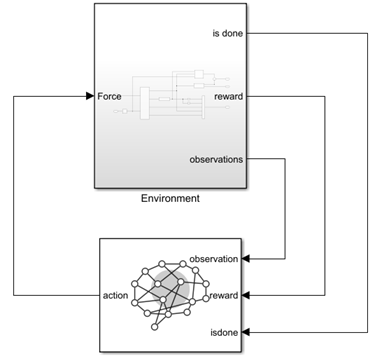

Simulink model of an environment in a feedback loop with an agent block.

In the Environment subsystem, the model dynamics are defined using Simscape components and the reward and observation are constructed using Simulink blocks.

open_system('rlCartPoleSimscapeModel/Environment')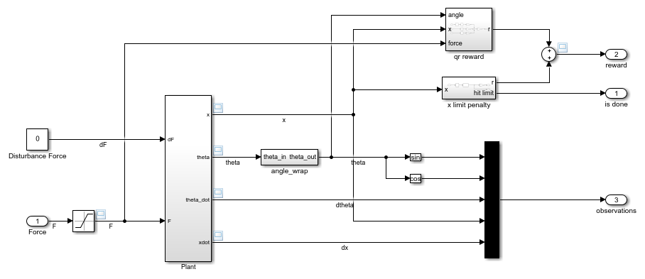

Simulink model of a cart-pole system.

There are two cart-pole environment variants, which differ by the agent action space.

Discrete — Agent can apply a force of 15, 0, or -15 to the cart.
Continuous — Agent can apply any force within the range [-15,15].

To create a cart-pole environment, use the rlPredefinedEnv function.

Discrete action space

env = rlPredefinedEnv('CartPoleSimscapeModel-Discrete');

Continuous action space

env = rlPredefinedEnv('CartPoleSimscapeModel-Continuous');

For an example that trains an agent in this cart-pole environment, see Train DDPG Agent to Swing Up and Balance Cart-Pole System.

Actions

In the cart-pole environments, the agent interacts with the environment using a single action signal, the force applied to the cart. The environment contains a specification object for this action signal. For the environment with a:

Discrete action space, the specification is an rlFiniteSetSpec object.
Continuous action space, the specification is an rlNumericSpec object.

For more information on obtaining action specifications from an environment, see getActionInfo.

Observations

In the cart-pole environment, the agent receives the following five observation signals.

Sine of the pole angle
Cosine of the pole angle
Derivative of the pendulum angle
Cart position
Derivative of cart position

For each observation signal, the environment contains an rlNumericSpec observation specification. All the observations are continuous and unbounded.

For more information on obtaining observation specifications from an environment, see getObservationInfo.

Reward

The reward signal for this environment is the sum of two components (r = r_qr + r_n + r_p):

A quadratic regulator control reward, constructed in the Environment/qr reward subsystem.

$r_{q r} = - (0.1 * x^{2} + 0.5 * θ^{2} + 0.005 * u_{t - 1}^{2})$
A cart limit penalty, constructed in the Environment/x limit penalty subsystem. This subsystem generates a negative reward when the magnitude of the cart position exceeds a given threshold.

$r_{p} = - 100 * (| x | \geq 3.5)$