Interactive Curve and Surface Fitting

Introducing Curve Fitter App

You can fit curves and surfaces to data and view plots with the Curve Fitter app.

Create, plot, and compare multiple fits.
Use linear or nonlinear regression, interpolation, smoothing, and custom equations.
View goodness-of-fit statistics, display confidence intervals and residuals, remove outliers, and assess fits with validation data.
Automatically generate code to fit and plot curves and surfaces, or export fits to the workspace for further analysis.

Fit Curve

Load some example data at the MATLAB^® command line.
```
load census
```
Open the Curve Fitter app.
```
curveFitter
```
Alternatively, on the Apps tab, in the Math, Statistics and Optimization group, click Curve Fitter.
On the Curve Fitter tab, in the Data section, click Select Data. In the Select Fitting Data dialog box, select cdate as the X data value and pop as the Y data value. For details, see Selecting Data to Fit in Curve Fitter App.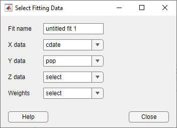
The Curve Fitter app creates a default polynomial fit to the data.
Try different fit options. For example, in the Fit Options pane, change the polynomial Degree value to 3 to fit a cubic polynomial.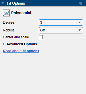
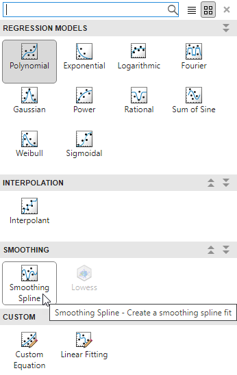
Select a different model type from the fit gallery in the Fit Type section on the Curve Fitter tab. For example, click the arrow to open the gallery, and click Smoothing Spline in the Smoothing group. For information about models you can fit, see Model Types for Curves and Surfaces.
In the Export section, click Export and select Generate Code.
The Curve Fitter app creates a file in the Editor containing MATLAB code to recreate the currently selected fit and its opened plots in your interactive session.

Tip

For a detailed workflow example, see Compare Fits in Curve Fitter App.

To create multiple fits and compare them, see Create Multiple Fits in Curve Fitter App.

Fit Surface

Load some example data at the MATLAB command line.
```
load franke
```
Open the Curve Fitter app.
```
curveFitter
```
On the Curve Fitter tab, in the Data section, click Select Data. In the Select Fitting Data dialog box, select x as the X data value, y as the Y data value, and z as the Z data value. For more information, see Selecting Data to Fit in Curve Fitter App.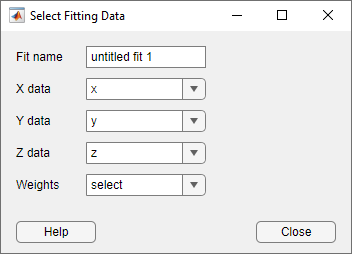
The Curve Fitter app creates a default interpolation fit to the data.
Select a different model type from the fit gallery in the Fit Type section on the Curve Fitter tab. For example, click the arrow to open the gallery, and click Polynomial in the Regression Models group.
For information about models you can fit, see Model Types for Curves and Surfaces.
Try different fit options for your chosen model type.
In the Export section, click Export and select Generate Code.
The Curve Fitter app creates a file in the Editor containing MATLAB code to recreate the currently selected fit and its opened plots in your interactive session.

Tip

For a detailed example, see Surface Fitting to Franke Data.

To create multiple fits and compare them, see Create Multiple Fits in Curve Fitter App.

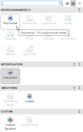
Model Types for Curves and Surfaces

Based on your selected data, the fit gallery shows either curve or surface fit groups. The following table describes the options for curves and surfaces.

Fit Group	Fit Type	Curves	Surfaces
Regression Models	Polynomial	Yes (up to degree 9)	Yes (up to degree 5)
	Exponential	Yes	No
	Fourier	Yes	No
	Gaussian	Yes	No
	Power	Yes	No
	Rational	Yes	No
	Sum of Sine	Yes	No
	Weibull	Yes	No
Interpolation	Interpolant	Yes, with methods: Nearest neighbor Linear Cubic Shape-preserving (PCHIP)	Yes, with methods: Nearest neighbor Linear Cubic Biharmonic (v4) Thin-plate spline
Smoothing	Smoothing Spline	Yes	No
Smoothing	Lowess	No	Yes
Custom	Custom Equation	Yes	Yes
Custom	Linear Fitting	Yes	No

For information about these fit types, see:

Selecting Data to Fit in Curve Fitter App

To select data to fit in the Curve Fitter app, click Select Data in the Data section on the Curve Fitter tab. You can select variables in your MATLAB workspace.

To fit curves:
- In the Select Fitting Data dialog box, select X data and Y data.
- Select only Y data to plot Y against the index X = 1:length(Y).
To fit surfaces, select X data, Y data, and Z data in the Select Fitting Data dialog box.

In the Select Fitting Data dialog box, you can use the drop-down lists to select any numeric variable in your MATLAB workspace that has more than one element. You can also select a numeric variable that is a column in a table variable. First select the table name, and then select the column name.

Similarly, you can select any numeric variable in your workspace to use as Weights, including a numeric table column.

Select Fitting Data dialog box with table variable selections

For curves, the X and Y variables must have the same number of elements. If you specify weights, the weights variable must have the same number of elements as the other data variables.

For surfaces, the X, Y, and Z variables must be either arrays with the same number of elements, or two vectors (X and Y) representing the row and column headers of a matrix Z. If you specify weights, the weights variable must have the same number of elements as the Z variable.

For more information, see Selecting Compatible Size Surface Data.

When you select variables, the Curve Fitter app immediately creates a curve or surface fit with the default settings. If you want to avoid time-consuming refitting for large data sets, you can turn off the automatic behavior. On the Curve Fitter tab, in the Fit section, select Manual.

Note

The Curve Fitter app uses a snapshot of the data you select. Subsequent workspace changes to the data have no effect on your fits. To update your fit data from the workspace, first change the variable selection, and then reselect the variable with the drop-down controls.

If there are problems with the data you select, you can see messages in the Results pane. For example, the Curve Fitter app ignores Infs, NaNs, and imaginary components of complex numbers in the data, and displays messages in the Results pane in these cases.

If you see warnings about reshaping your data or incompatible sizes, read Selecting Compatible Size Surface Data and Troubleshooting Data Problems for more information.

Save and Reopen Sessions

You can save and reopen sessions for easy access to multiple fits. The session file contains all the fits and variables in your session and remembers your layout.

To save your session, first click the Save button in the File section on the Curve Fitter tab to open your file browser. Next, select a name and location for your session file (with the file extension .sfit).

After you save your session once, you can click Save and select Save Session to overwrite that session with subsequent saves.

To save the current session under a different name, click Save and select Save Session As.

To reopen a session, click Open in the File section on the Curve Fitter tab to open a file browser where you can select a saved curve fitting session file to load.