Simulate DC Motor Step Response Using Local Solver

Open Live Script

This example shows how using a local solver can improve simulation performance for a model hierarchy that contains components that operate on different time scales. The model in this example simulates the step response of a DC motor driving a mechanical load.

A DC Motor is represented as an electrical and mechanical diagram. The electrical diagram includes a voltage source driving a resistor and inductor in series

Subcomponents of dynamic systems can operate on different time scales. For example, in this DC motor model, the electrical physics of the step response operate on a time scale close to a microsecond, while the mechanical motion occurs on a time scale of miliseconds.

When you use referenced models to represent system components, you can configure the referenced models to use local solvers. For example, the referenced model that represents the mechanical motion can run with a larger solver step size than the rest of the DC motor model.

Analyze System Dynamics

To determine whether your system might benefit from using a local solver, analyze the dynamics of your system. Local solvers can provide performance improvements by increasing the step size for components with slower dynamics compared to other parts of the system or allowing you to use a different solver that is better suited to that component.

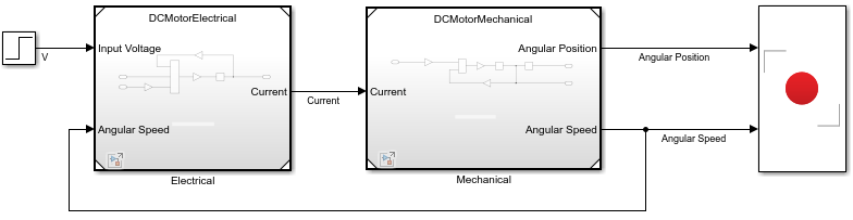
Open the model DCMotorLocalSolver. The model implements the system using two referenced models:

The model DCMotorElectrical models the electrical response of the motor.
The model DCMotorMechanical models the mechanical response of the motor.

The electrical and mechanical systems are coupled by the motor current and the angular speed of the motor and load.

topMdl = "DCMotorLocalSolver";
mechRef = "DCMotorMechanical";
elecRef = "DCMotorElectrical";

open_system(topMdl)
load_system(mechRef)
load_system(elecRef)

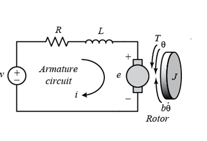
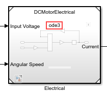
The model DCMotorLocalSolver contains two Model blocks, Electrical and Mechanical. A Step block provides input to the Electrical Model block, which sends a signal named Current to the Mechanical Model block. A Record block logs and plots data for the Angular Position and Angular Speed signals.

To analyze the electrical component, open the referenced model named DCMotorElectrical in the Simulink™ Editor by double-clicking the Model block named Electrical. The electrical dynamics of the motor are modeled as a series RL circuit.

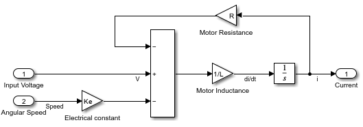
The block diagram models the electrical dynamics of the motor using the motor electrical constant, resistance, and inductance. The inputs are the input voltage and angular speed, and the output is the motor current.

The input voltage $v$ can be expressed as the sum of the voltage on the motor resistance $iR$ , the voltage on the motor inductance $L \frac{di}{dt}$ , and the voltage due to the motor electrical constant $K_{e}$ and the angular velocity $\frac{d θ}{dt}$ .

$v = iR + L \frac{d i}{d t} + K_{e} \frac{d θ}{d t}$

The electrical component in the model calculates the value of the current, which the mechanical system uses to calculate the speed of the motor and load.

$\frac{d i}{d t} = \frac{v}{L} - \frac{R}{L} i - \frac{K_{e}}{L} \frac{d θ}{d t}$

The motor inductance and resistance determine the electrical time constant $t_{e}$ for the system.

$t_{e} = \frac{L}{R}$

The motor in this model has an inductance of $2.5 μ H$ and a resistance of $3 Ω$ , resulting in an electrical time constant of $200 ns$ .

To analyze the mechanical component, navigate back to the top model by clicking the back arrow . Then, open the referenced model named DCMotorMechanical in the Simulink Editor by double-clicking the Model block named Mechanical.

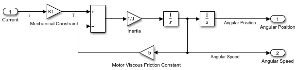
The mechanical system models the rotational motion that results from the torque produced by the motor current. The total rotational moment of inertia from the motor and the load $J$ times the angular acceleration $\frac{d θ}{d t^{2}}$ is equal to the sum of the forces in the system. The motor current $i$ and the magnetic field in the armature coil create a force scaled by the motor torque constant $K_{T}$ . For this example, assume the magnetic field is constant. The angular speed $\frac{d Ɵ}{d t}$ creates a force scaled by the viscous friction of the motor $b$ .

$J \frac{d θ}{d t^{2}} = K_{T} i - b \frac{d Ɵ}{d t}$

The mechanical component in the model integrates the angular acceleration to calculate the angular speed of the motor and load, which the electrical system uses to calculate the current.

$\frac{d θ}{d t^{2}} = \frac{K_{T}}{J} i - \frac{b}{J} \frac{d Ɵ}{d t}$

The motor resistance, the inertia of the motor and load, the electrical constant, and the torque constant for the motor determine the mechanical time constant $t_{m}$ [1].

$t_{m} = \frac{R J}{K_{e} K_{T}}$

The motor in this model has a resistance of $3 Ω$ , an electrical constant of $0.025 \frac{Vs}{rad}$ , and a torque constant of $0.25 \frac{Nm}{A}$ . The total moment of inertia for the system is $3.2 μ Nm s^{2}$ , resulting in a mechanical time constant of $15.4 ms$ .

Run Baseline Simulation

Simulate the model using a single solver to create a baseline for the simulation outputs and timing. Using a single solver, the whole system must run using the same time step. The electrical time constant drives the choice of the step size. The step size must be small enough to capture the dynamics of the electrical response.

For this example, the model uses the ode3 fixed-step solver with a step size equal to the electrical time constant, $200 ns$ . Simulate the model to create a baseline for the simulation results and execution time.

set_param(mechRef,"UseModelRefSolver","off")
baselineOut = sim(topMdl);

To see the amount of time required to execute the simulation, check the ExecutionElaspedWallTime field of the TimingInfo structure in the simulation metadata. The Simulink.SimulationOutput object baselineOut contains a Simulink.SimulationMetadata object with information about the model and simulation, including the structure TimingInfo.

Using a single configuration for the ode3 solver with a step size of $200 ns$ , the execution phase of the simulation runs for several seconds.

baseExec = baselineOut.SimulationMetadata.TimingInfo.ExecutionElapsedWallTime

baseExec = 3.6396

The Record block in the model logs the position and speed data to the Simulation Data Inspector. Access the run created in the Simulation Data Inspector and change the name to Baseline: DCMotorLocalSolver.

baseRun = Simulink.sdi.Run.getLatest;
baseRun.Name = "Baseline: DCMotorLocalSolver";

Simulate Using Local Solver

To see the performance benefit and impact on the model outputs, configure the mechanical model to use a local solver. The dynamics of the mechanical system operate on a longer time scale. When you configure the model to use a local solver, you can specify a larger time step so that the mechanical system calculations do not occur more frequently than required for capturing the system response.

In the top model, continue to use the $200 ns$ step size. Configure the DCMotorMechanical model to use the ode3 solver as a local solver with a step size of 2ms. You can configure the settings for the model reference from the top model, using the Property Inspector or the Block Parameters dialog box.

In the top model, select the Model block that references the DCMotorMechanical model.
Open the Property Inspector. On the Modeling tab, expand the Design section and select Property Inspector, or press Ctrl+Shift+I.
In the Property Inspector, expand the Solver section.
Click the hyperlink next to the Use local solver parameter. The Configuration Parameters dialog box for the referenced model opens.
In the Configuration Parameters dialog box for the DCMotorMechanical model, on the Model Referencing pane, select Use local solver when referencing model.
To configure the solver settings for the referenced model, select the Solver pane.
Set the Solver to ode3 (Bogacki-Shampine).
Set the Fixed step size (fundamental sample time) to 0.002.
Click OK.

In the model, the Model block indicates the local solver selected for the referenced model.

The Model block has a label that says ode3 to indicate that the referenced model is configured to use the ode3 solver as a local solver.

Alternatively, you can configure the model settings programmatically using the set_param function.

set_param(mechRef,"UseModelRefSolver","on","SolverType","Fixed-step",...
    "Solver","ode3","FixedStep","0.002");

The Model block parameters Input signal handling and Output signal handling specify how the local solver processes inputs from the top model and provides outputs to the top model. For this simulation, use the default values.

mdlBlkPath = append(topMdl,"/Mechanical");
set_param(mdlBlkPath,"InputSignalHandling","Auto",...
    "OutputSignalHandling","Use solver interpolant")

Simulate the model using the local solver.

localOut = sim(topMdl);

Check the simulation metadata to see the amount of time the simulation spent in the execution phase. When you use a local solver to execute the mechanical system at a slower rate, the simulation runs faster.

localExec = localOut.SimulationMetadata.TimingInfo.ExecutionElapsedWallTime

localExec = 2.4772

Access the run created in the Simulation Data Inspector. Change the name to Local Solver: DCMotorLocalSolver.

localRun = Simulink.sdi.Run.getLatest;
localRun.Name = "LocalSolver: DCMotorLocalSolver";

Analyze Simulation Results

To see whether using a local solver affected the simulation results, plot the position and speed data from both simulations in the Simulation Data Inspector.

On the Simulation tab, under Review Results, click Data Inspector. Alternatively, use the Simulink.sdi.view function.

Simulink.sdi.view

In the Simulation Data Inspector, plot the speed and position signals from the two runs. Alternatively, use the Simulink.sdi.loadView function to load the saved view for this example, which is named DCMotorLocalSolver1.

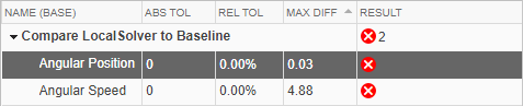
Simulink.sdi.loadView("DCMotorLocalSolver1");

The results from the local solver simulation are nearly the same as the results from the baseline simulation that used a single solver and step size. The solid line shows the baseline result. The dotted line shows the local solver result.

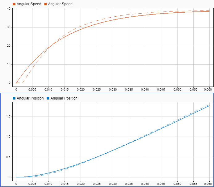
A two-by-one plot in the Simulation Data Inspector shows the Angular Speed signals from the baseline and local solver simulations on the top plot and the angular position signal from the two simulations on the bottom plot.

The biggest difference occurs in the Angular Speed signal at the start of the simulation. The local solver determines required state and signal values from the top model using extrapolation. The first time the local solver takes a step, the local solver does not have enough history for extrapolation. On the second step, the local solver can extrapolate values from the top model and compensate in the output value.

Use Zero-Order Hold Input and Output Handling

Because the execution of the local solver is decoupled from the top solver, the local solver extrapolates values it uses from the top model and provides interpolated values for the top solver to use. You can use the Input signal handling and Output signal handling to configure how the local solver extrapolates the incoming and inteprolates outgoing values.

By default, the Input signal handling parameter value is Auto. The software determines how to extrapolate the data that the local solver uses from the top model. The default value for the Output signal handling parameter is Use solver interpolant, which means that the local solver provides output values that are compensated using the solver interpolant.

You can specify each parameter as Zero-order hold instead. Configure the Model block that references the DCMotorMechanical model to use Zero-order hold input and output signal handling.

set_param(mdlBlkPath,"InputSignalHandling","Zero-order hold",...
    "OutputSignalHandling","Zero-order hold")

To see the effect of the input and output signal handling on the simulation results, simulate the model again.

zohOut = sim(topMdl);

Check the execution time for the simulation. Using the simpler extrapolation method further reduces the execution time.

zohExec = zohOut.SimulationMetadata.TimingInfo.ExecutionElapsedWallTime

zohExec = 3.3558

Access the run created in the Simulation Data Inspector. Change the name to Local Solver ZOH: DCMotorMechanical.

zohRun = Simulink.sdi.Run.getLatest;
zohRun.Name = "Local Solver ZOH: DCMotorMechanical";

The Simulation Data Inspector replaces the signals from the first local solver run with the signals from the zero-order hold run. The signal values are similar between the baseline run and the zero-order hold run. The signals from the zero-order hold run have steps that reflect the zero-order hold and the step size for the local solver.

Reference

[1] Younkin, George W. "Electric Servo Motor Equations and Time Constants." https://support.controltechnologycorp.com/customer/elearning/younkin/driveMotorEquations.pdf.

Simulate DC Motor Step Response Using Local Solver

Analyze System Dynamics

Run Baseline Simulation

Simulate Using Local Solver

Analyze Simulation Results

Use Zero-Order Hold Input and Output Handling

Reference

See Also

Blocks

Model Settings

Related Topics