Train Multiple Agents for Area Coverage

Create Environment

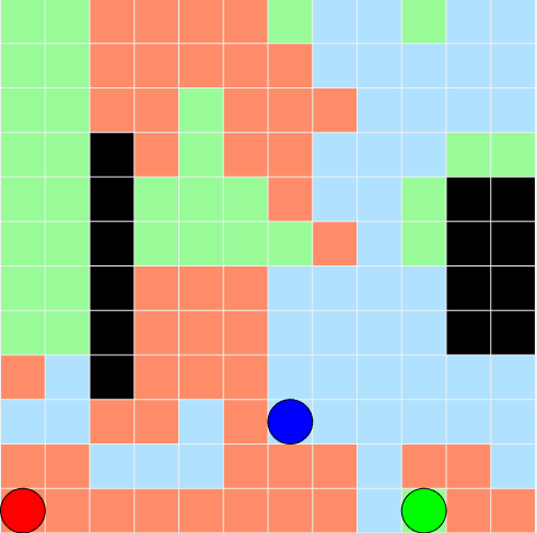
The environment in this example is a 12x12 grid world containing obstacles, with unexplored cells marked in white and obstacles marked in black. There are three robots in the environment represented by the red, green, and blue circles. Three proximal policy optimization agents with discrete action spaces control the robots. To learn more about PPO agents, see Proximal Policy Optimization (PPO) Agents.

The agents provide one of five possible movement actions (WAIT, UP, DOWN, LEFT, or RIGHT) to their respective robots. The robots decide whether an action is legal or illegal. For example, an action of moving LEFT when the robot is located next to the left boundary of the environment is deemed illegal. Similarly, actions for colliding against obstacles and other agents in the environment are illegal actions and draw penalties. The environment dynamics are deterministic, which means the robots execute legal and illegal actions with 100% and 0% probabilities, respectively. The overall goal is to explore all cells as quickly as possible.

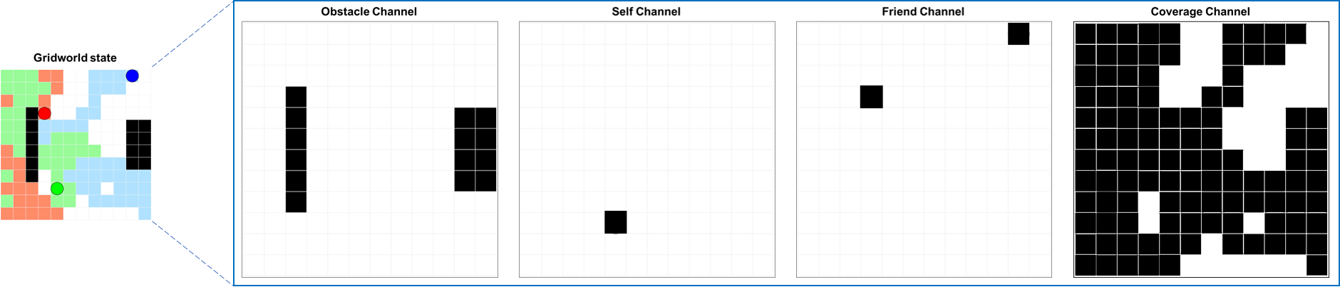
At each time step, an agent observes the state of the environment through a set of four images that identify the cells with obstacles, current position of the robot that is being controlled, position of other robots, and cells that have been explored during the episode. These images are combined to create a 4-channel 12x12 image observation set. The following figure shows an example of what the agent controlling the green robot observes for a given time step.

For the grid world environment:

At each time step, agents receive the following rewards and penalties.

Define the locations of obstacles within the grid using a matrix of indices. The first column contains the row indices, and the second column contains the column indices.

obsMat = [4 3; 5 3; 6 3; 7 3; 8 3; 9 3; 5 11; 
    6 11; 7 11; 8 11; 5 12; 6 12; 7 12; 8 12];

Initialize the robot positions.

sA0 = [2 2];
sB0 = [11 4];
sC0 = [3 12];
s0 = [sA0; sB0; sC0];

Specify the sample time, simulation time, and maximum number of steps per episode.

Ts = 0.1;
Tf = 100;
maxsteps = ceil(Tf/Ts);

Open the Simulink model.

mdl = "rlAreaCoverage";
open_system(mdl)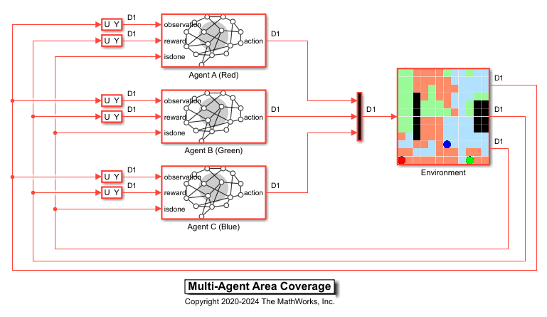

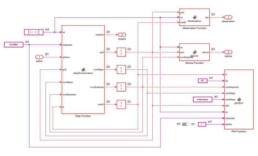
The GridWorld block is a MATLAB System block representing the training environment. The System object for this environment is defined in GridWorld.m.

In this example, the agents are homogeneous and have the same observation and action specifications. Create the observation and action specifications for the environment. For more information, see rlNumericSpec and rlFiniteSetSpec.

% Define observation specifications.
obsSize = [12 12 4];
oinfo = rlNumericSpec(obsSize);
oinfo.Name = "observations";

% Define action specifications.
numAct = 5;
actionSpace = {0,1,2,3,4};
ainfo = rlFiniteSetSpec(actionSpace);
ainfo.Name = "actions";

Specify the block paths for the agents.

blks = mdl + ["/Agent A (Red)","/Agent B (Green)","/Agent C (Blue)"];

Create the environment interface, specifying the same observation and action specifications for all three agents.

env = rlSimulinkEnv(mdl,blks,{oinfo,oinfo,oinfo},{ainfo,ainfo,ainfo});

Specify a reset function for the environment. The reset function resetMap ensures that the robots start from random initial positions at the beginning of each episode. The random initialization makes the agents robust to different starting positions and improves training convergence.

env.ResetFcn = @(in) resetMap(in, obsMat);

Create Agents

The PPO agents in this example operate on a discrete action space and rely on actor and critic functions to learn the optimal policies. The agents maintain deep neural network-based function approximators for the actors and critics with similar network structures (a combination of convolution and fully connected layers). The critic outputs a scalar value representing the state value $\mathit{V}\left(\mathit{s}\right)$. The actor outputs the probabilities $\pi \left(\mathit{a}|\mathit{s}\right)$ of taking each of the five actions WAIT, UP, DOWN, LEFT, or RIGHT.

Set the random seed for reproducibility.

rng(0)

Create the actor and critic functions using the following steps.

Use the same network structure and representation options for all three agents.

for idx = 1:3

    % Create actor deep neural network.
    actorNetWork = [
        imageInputLayer(obsSize,Normalization="none")
        convolution2dLayer(8,16, ...
            Stride=1,Padding=1,WeightsInitializer="he")
        reluLayer
        convolution2dLayer(4,8, ...
            Stride=1,Padding="same",WeightsInitializer="he")
        reluLayer
        fullyConnectedLayer(256,WeightsInitializer="he")
        reluLayer
        fullyConnectedLayer(128,WeightsInitializer="he")
        reluLayer
        fullyConnectedLayer(64,WeightsInitializer="he")
        reluLayer
        fullyConnectedLayer(numAct)
        softmaxLayer
        ];
    actorNetWork = dlnetwork(actorNetWork);
    
    % Create critic deep neural network.
    criticNetwork = [
        imageInputLayer(obsSize,Normalization="none")
        convolution2dLayer(8,16, ...
            Stride=1,Padding=1,WeightsInitializer="he")
        reluLayer
        convolution2dLayer(4,8, ...
            Stride=1,Padding="same",WeightsInitializer="he")
        reluLayer
        fullyConnectedLayer(256,WeightsInitializer="he")
        reluLayer
        fullyConnectedLayer(128,WeightsInitializer="he")
        reluLayer
        fullyConnectedLayer(64,WeightsInitializer="he")
        reluLayer
        fullyConnectedLayer(1)
        ];
    criticNetwork = dlnetwork(criticNetwork);
    
    % create actor and critic
    actor(idx) = rlDiscreteCategoricalActor(actorNetWork,oinfo,ainfo);
    critic(idx) = rlValueFunction(criticNetwork,oinfo);
end

Specify training options for the critic and the actor using rlOptimizerOptions.

actorOpts = rlOptimizerOptions(LearnRate=1e-4,GradientThreshold=1);
criticOpts = rlOptimizerOptions(LearnRate=1e-4,GradientThreshold=1);

Specify the agent options using rlPPOAgentOptions, include the training options for the actor and critic. Use the same options for all three agents. During training, agents collect experiences until they reach the experience horizon of 128 steps and then train from mini-batches of 64 experiences. An objective function clip factor of 0.2 improves training stability, and a discount factor value of 0.995 encourages long-term rewards.

opt = rlPPOAgentOptions(...
    ActorOptimizerOptions=actorOpts,...
    CriticOptimizerOptions=criticOpts,...
    ExperienceHorizon=128,...
    ClipFactor=0.2,...
    EntropyLossWeight=0.01,...
    MiniBatchSize=64,...
    NumEpoch=3,...
    AdvantageEstimateMethod="gae",...
    GAEFactor=0.95,...
    SampleTime=Ts,...
    DiscountFactor=0.995);

Create the agents using the defined actors, critics, and options.

agentA = rlPPOAgent(actor(1),critic(1),opt);
agentB = rlPPOAgent(actor(2),critic(2),opt);
agentC = rlPPOAgent(actor(3),critic(3),opt);

Alternatively, you can create the agents first, and then access their option object to modify the options using dot notation.

Train Agents

In this example, the agents are trained independently in decentralized manner. Specify the following options for training the agents.

trainOpts = rlMultiAgentTrainingOptions(...
    "AgentGroups","auto",...
    "LearningStrategy","decentralized",...
    MaxEpisodes=1000,...
    MaxStepsPerEpisode=maxsteps,...
    Plots="training-progress",...
    ScoreAveragingWindowLength=100,...
    StopTrainingCriteria="AverageReward",...
    StopTrainingValue=80); 

For more information on multi-agent training, type help rlMultiAgentTrainingOptions in MATLAB.

To train the agents, specify an array of agents to the train function. The order of the agents in the array must match the order of agent block paths specified during environment creation. Doing so ensures that the agent objects are linked to the appropriate action and observation specifications in the environment.

Training is a computationally intensive process that takes several minutes to complete. To save time while running this example, load pretrained agent parameters by setting doTraining to false. To train the agent yourself, set doTraining to true.

doTraining = false;
if doTraining
    result = train([agentA,agentB,agentC],env,trainOpts);
else
    load("rlAreaCoverageAgents.mat");
end

The following figure shows a snapshot of the training progress. You can expect different results due to randomness in the training process.

Simulate Agents

Simulate the trained agents within the environment. For more information on agent simulation, see rlSimulationOptions and sim.

rng(0) % reset the random seed
simOpts = rlSimulationOptions(MaxSteps=maxsteps);
experience = sim(env,[agentA,agentB,agentC],simOpts);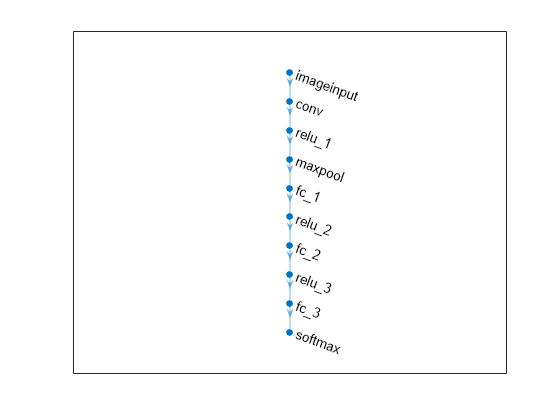

The agents successfully cover the entire grid world.