Train DQN Agent to Balance Cart-Pole System

Cart-Pole MATLAB Environment

The reinforcement learning environment for this example is a pole attached to an unactuated joint on a cart, which moves along a frictionless track. The training goal is to make the pole stand upright without falling over.

For this environment:

For more information on this model, see Load Predefined Control System Environments.

Create Environment Interface

Create a predefined environment interface for the system.

env = rlPredefinedEnv("CartPole-Discrete")

env = 
  CartPoleDiscreteAction with properties:

                  Gravity: 9.8000
                 MassCart: 1
                 MassPole: 0.1000
                   Length: 0.5000
                 MaxForce: 10
                       Ts: 0.0200
    ThetaThresholdRadians: 0.2094
               XThreshold: 2.4000
      RewardForNotFalling: 1
        PenaltyForFalling: -5
                    State: [4x1 double]

The interface has a discrete action space where the agent can apply one of two possible force values to the cart, –10 or 10 N.

Get the observation and action specification information.

obsInfo = getObservationInfo(env)

obsInfo = 
  rlNumericSpec with properties:

     LowerLimit: -Inf
     UpperLimit: Inf
           Name: "CartPole States"
    Description: "x, dx, theta, dtheta"
      Dimension: [4 1]
       DataType: "double"

actInfo = getActionInfo(env)

actInfo = 
  rlFiniteSetSpec with properties:

       Elements: [-10 10]
           Name: "CartPole Action"
    Description: [0x0 string]
      Dimension: [1 1]
       DataType: "double"

Fix the random generator seed for reproducibility.

rng(0)

Create DQN Agent

DQN agents can use vector Q-value functions critics, which are generally more efficient than comparable single-output critics. A vector Q-value function critic has observations as inputs and state-action values as outputs. Each output element represents the expected cumulative long-term reward for taking the corresponding discrete action from the state indicated by the observation inputs. For more information on creating value-functions, see Create Policies and Value Functions.

To approximate the Q-value function within the critic, use a neural network with one input channel (the 4-dimensional observed state vector) and one output channel with two elements (one for the 10 N action, another for the –10 N action). Define the network as an array of layer objects, and get the dimension of the observation space and the number of possible actions from the environment specification objects.

net = [
    featureInputLayer(obsInfo.Dimension(1))
    fullyConnectedLayer(20)
    reluLayer
    fullyConnectedLayer(length(actInfo.Elements))
    ];

Convert to dlnetwork and display the number of weights.

net = dlnetwork(net);
summary(net)

   Initialized: true

   Number of learnables: 142

   Inputs:
      1   'input'   4 features

View the network configuration.

plot(net)

Create the critic approximator using net and the environment specifications. For more information, see rlVectorQValueFunction.

critic = rlVectorQValueFunction(net,obsInfo,actInfo);

Check the critic with a random observation input.

getValue(critic,{rand(obsInfo.Dimension)})

ans = 2x1 single column vector

   -0.2257
    0.4299

Create the DQN agent using critic. For more information, see rlDQNAgent.

agent = rlDQNAgent(critic);

Check the agent with a random observation input.

getAction(agent,{rand(obsInfo.Dimension)})

ans = 1x1 cell array
    {[10]}

Specify the DQN agent options, including training options for the critic. Alternatively, you can use rlDQNAgentOptions and rlOptimizerOptions objects.

agent.AgentOptions.UseDoubleDQN = false;
agent.AgentOptions.TargetSmoothFactor = 1;
agent.AgentOptions.TargetUpdateFrequency = 4;
agent.AgentOptions.ExperienceBufferLength = 1e5;
agent.AgentOptions.MiniBatchSize = 256;
agent.AgentOptions.CriticOptimizerOptions.LearnRate = 1e-3;
agent.AgentOptions.CriticOptimizerOptions.GradientThreshold = 1;

Train Agent

To train the agent, first specify the training options. For this example, use the following options:

For more information, see rlTrainingOptions.

trainOpts = rlTrainingOptions(...
    MaxEpisodes=1000, ...
    MaxStepsPerEpisode=500, ...
    Verbose=false, ...
    Plots="training-progress",...
    StopTrainingCriteria="AverageReward",...
    StopTrainingValue=480); 

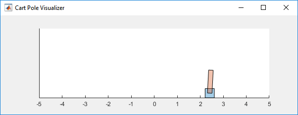
You can visualize the cart-pole system by using the plot function during training or simulation.

plot(env)

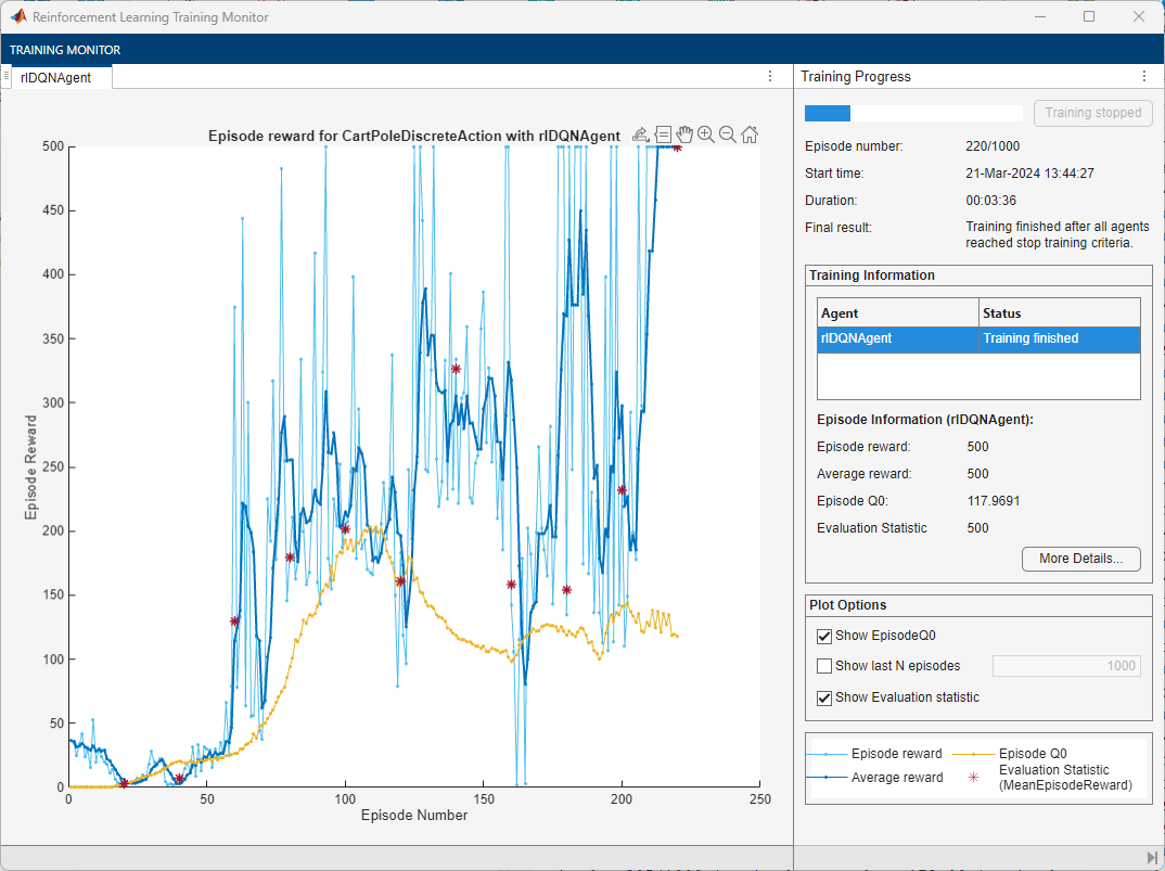
Train the agent using the train function. Training this agent is a computationally intensive process that takes several minutes to complete. To save time while running this example, load a pretrained agent by setting doTraining to false. To train the agent yourself, set doTraining to true.

doTraining = false;
if doTraining
    % Train the agent.
    trainingStats = train(agent,env,trainOpts);
else
    % Load the pretrained agent for the example.
    load("MATLABCartpoleDQNMulti.mat","agent")
end

Simulate DQN Agent

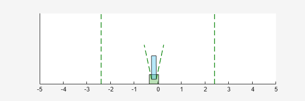
To validate the performance of the trained agent, simulate it within the cart-pole environment. For more information on agent simulation, see rlSimulationOptions and sim. The agent can balance the cart-pole even when the simulation time increases to 500 steps.

simOptions = rlSimulationOptions(MaxSteps=500);
experience = sim(env,agent,simOptions);

totalReward = sum(experience.Reward)

totalReward = 500