Water Distribution System Scheduling Using Reinforcement Learning

This example uses:

This example shows how to learn an optimal pump scheduling policy for a water distribution system using reinforcement learning (RL).

Water Distribution System

The following figure shows a water distribution system.

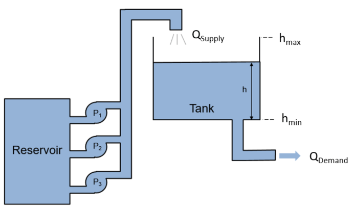
Here:

$Q_{Supply}$ is the amount of water supplied to the water tank from a reservoir.
$Q_{Demand}$ is the amount of water flowing out of the tank to satisfy usage demand.

The objective of the reinforcement learning agent is to schedule the number of pumps running to both minimize the energy usage of the system and satisfy the usage demand ( $h > 0$ ). The dynamics of the tank system are governed by the following equation.

$A \frac{dh}{dt} = Q_{Supply} (t) - Q_{Demand} (t)$

Here, $A = 40 m^{2}$ and $h_{\max} = 7 m$ . The demand over a 24 hour period is a function of time given as

$Q_{Demand} (t) = μ (t) + η (t)$

where $μ (t)$ is the expected demand and $η (t)$ represents the demand uncertainty, which is sampled from a uniform random distribution.

The supply is determined by the number of pumps running, $a \in {0, 1, 2, 3}$ according to following mapping.

$Q_{Supply} (t) = Q (a) = {\begin{cases} 0 & a = 0 \\ 164 & a = 1 \\ 279 & a = 2 \\ 344 & a = 3 \end{cases} \frac{cm}{h}$

To simplify the problem, power consumption is defined as the number of pumps running, $a$ .

The following function is the reward for this environment. To avoid overflowing or emptying the tank, an additional cost is added if the water height is close to the maximum or minimum water levels, $h_{\max}$ or $h_{\min}$ , respectively.

$r (h, a) = - 10 (h \geq (h_{\max} - 0.1)) - 10 (h \leq 0.1) - a$

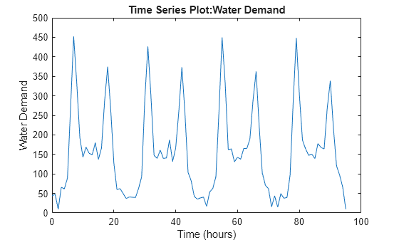
Generate Demand Profile

To generate and a water demand profile based on the number of days considered, use the generateWaterDemand function defined at the end of this example.

num_days = 4; % Number of days
[WaterDemand,T_max] = generateWaterDemand(num_days);

View the demand profile.

plot(WaterDemand)

Figure contains an axes object. The axes object with title Time Series Plot:Water Demand, xlabel Time (hours), ylabel Water Demand contains an object of type line.

Open and Configure Model

Open the distribution system Simulink model.

mdl = "watertankscheduling";
open_system(mdl)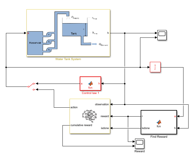

In addition to the reinforcement learning agent, a simple baseline controller is defined in the Control law MATLAB Function block. This controller activates a certain number of pumps depending on the water level.

Specify the initial water height.

h0 = 3; % m

Specify the model parameters.

SampleTime = 0.2;
H_max = 7; % Max tank height (m)
A_tank = 40; % Area of tank (m^2)

Create Environment Interface for RL Agent

To create an environment interface for the Simulink model, first define the action and observation specifications, actInfo and obsInfo, respectively. The agent action is the selected number of pumps. The agent observation is the water height, which is measured as a continuous-time signal.

actInfo = rlFiniteSetSpec([0,1,2,3]);
obsInfo = rlNumericSpec([1,1]);

Create the environment interface.

env = rlSimulinkEnv(mdl,mdl+"/RL Agent",obsInfo,actInfo);

Specify a custom reset function, which is defined at the end of this example, that randomizes the initial water height and the water demand. Doing so allows the agent to be trained on different initial water levels and water demand functions for each episode.

env.ResetFcn = @(in)localResetFcn(in);

The actor and critic networks are initialized randomly. Ensure reproducibility by fixing the seed of the random generator.

rng(0);

Create DQN Agent

DQN agents use a parametrized Q-value function approximator to estimate the value of the policy. Since DQN agents have a discrete action space, you have the option to create a vector (that is multi-output) Q-value function critic, which is generally more efficient than a comparable single-output critic.

A vector Q-value function takes only the observation as input and returns as output a single vector with as many elements as the number of possible actions. The value of each output element represents the expected discounted cumulative long-term reward when an agent starts from the state corresponding to the given observation and executes the action corresponding to the element number (and follows a given policy afterwards)

To model the parametrized Q-value function within the critic, use a non-recurrent neural network. To use a recurrent neural network, set useLSTM to true. Note that prod(obsInfo.Dimension) returns the number of dimensions of the observation space (regardless of whether they are arranged as a row vector, column vector, or matrix, while numel(actInfo.Elements) returns the number of elements of the discrete action space.

useLSTM = false;
if useLSTM
    layers = [
        sequenceInputLayer(prod(obsInfo.Dimension))
        fullyConnectedLayer(32)
        reluLayer
        lstmLayer(32)
        fullyConnectedLayer(32)
        reluLayer
        fullyConnectedLayer(numel(actInfo.Elements))
        ];
else
    layers = [
        featureInputLayer(obsInfo.Dimension(1))
        fullyConnectedLayer(32)
        reluLayer
        fullyConnectedLayer(32)
        reluLayer
        fullyConnectedLayer(32)
        reluLayer
        fullyConnectedLayer(numel(actInfo.Elements))
        ];
end

Convert to a dlnetwork object and display the number of parameters.

dnn = dlnetwork(layers);
summary(dnn)

   Initialized: true

   Number of learnables: 2.3k

   Inputs:
      1   'input'   1 features

Create a critic using rlVectorQValueFunction using the defined deep neural network and the environment specifications.

critic = rlVectorQValueFunction(dnn,obsInfo,actInfo);

Create DQN Agent

Specify training options for the critic and the actor using rlOptimizerOptions.

criticOpts = rlOptimizerOptions(LearnRate=0.001,GradientThreshold=1);

Specify the DDPG agent options using rlDQNAgentOptions. If you are using an LSTM network, set the sequence length to 20.

opt = rlDQNAgentOptions(SampleTime=SampleTime); 
if useLSTM
    opt.SequenceLength = 20;
else
    opt.SequenceLength = 1;
end
opt.DiscountFactor = 0.995;
opt.ExperienceBufferLength = 1e6;
opt.EpsilonGreedyExploration.EpsilonDecay = 1e-5;
opt.EpsilonGreedyExploration.EpsilonMin = .02;

Include the training options for the critic.

opt.CriticOptimizerOptions = criticOpts;

Create the agent using the critic and the options object.

agent = rlDQNAgent(critic,opt);

Train Agent

To train the agent, first specify the training options. For this example, use the following options.

Run training for 1000 episodes, with each episode lasting at ceil(T_max/Ts) time steps.
Display the training progress in the Episode Manager dialog box (set the Plots option)

Specify the options for training using an rlTrainingOptions object.

trainOpts = rlTrainingOptions(...
    MaxEpisodes=1000, ...
    MaxStepsPerEpisode=ceil(T_max/SampleTime), ...
    Verbose=false, ...
    Plots="training-progress",...
    StopTrainingCriteria="EpisodeCount",...
    StopTrainingValue=1000,...
    ScoreAveragingWindowLength=100);

While you do not do it for this example, you can save agents during the training process. For example, the following options save every agent with a reward value greater than or equal to -42.

Save agents using SaveAgentCriteria if necessary
trainOpts.SaveAgentCriteria = "EpisodeReward";
trainOpts.SaveAgentValue = -42;

Train the agent using the train function. Training this agent is a computationally intensive process that takes several hours to complete. To save time while running this example, load a pretrained agent by setting doTraining to false. To train the agent yourself, set doTraining to true.

doTraining = false;
if doTraining

    % Connect the RL Agent block by toggling 
    % the Manual Switch block
    set_param(mdl+"/Manual Switch","sw","0");

    % Train the agent.
    trainingStats = train(agent,env,trainOpts);
else
    % Load the pretrained agent for the example.
    load("SimulinkWaterDistributionDQN.mat","agent")
end

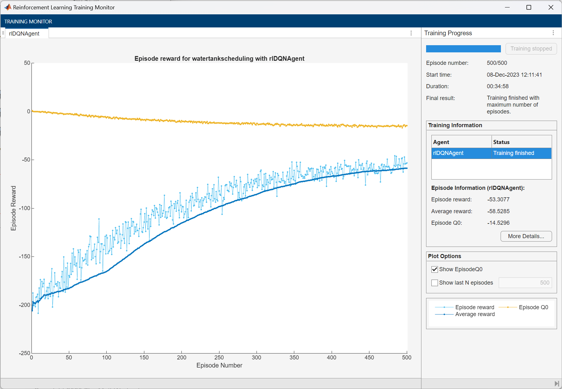
The following figure shows the training progress.

Simulate DQN Agent

To validate the performance of the trained agent, simulate it in the water-tank environment. For more information on agent simulation, see rlSimulationOptions and sim.

To simulate the agent performance, connect the RL Agent block by toggling the manual switch block.

set_param(mdl+"/Manual Switch","sw","0");

Set the maximum number of steps for each simulation and the number of simulations. For this example, run 30 simulations. The environment reset function sets a different initial water height and water demand are different in each simulation.

NumSimulations = 30;
simOptions = rlSimulationOptions(MaxSteps=T_max/SampleTime,...
    NumSimulations= NumSimulations);

To compare the agent with the baseline controller under the same conditions, reset the initial random seed used in the environment reset function.

env.ResetFcn("Reset seed");

Simulate the agent against the environment.

experienceDQN = sim(env,agent,simOptions);

Simulate Baseline Controller

To compare DQN agent with the baseline controller, you must simulate the baseline controller using the same simulation options and initial random seed for the reset function.

Enable the baseline controller.

set_param(mdl+"/Manual Switch","sw","1");

To compare the agent with the baseline controller under the same conditions, reset the random seed used in the environment reset function.

env.ResetFcn("Reset seed");

Simulate the baseline controller against the environment.

experienceBaseline = sim(env,agent,simOptions);

Compare DQN Agent with Baseline Controller

Initialize cumulative reward result vectors for both the agent and baseline controller.

resultVectorDQN = zeros(NumSimulations, 1);
resultVectorBaseline = zeros(NumSimulations,1);

Calculate cumulative rewards for both the agent and the baseline controller.

for ct = 1:NumSimulations
    resultVectorDQN(ct) = sum(experienceDQN(ct).Reward);
    resultVectorBaseline(ct) = sum(experienceBaseline(ct).Reward);
end

Plot the cumulative rewards.

plot([resultVectorDQN resultVectorBaseline],"o")
set(gca,"xtick",1:NumSimulations)
xlabel("Simulation number")
ylabel("Cumulative Reward")
legend("DQN","Baseline","Location","NorthEastOutside")

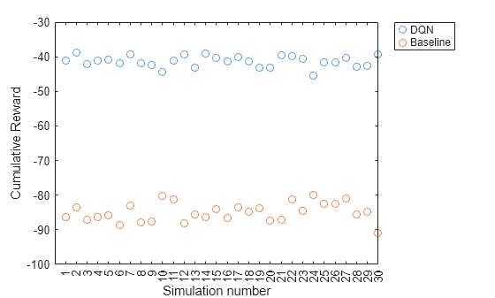
Figure contains an axes object. The axes object with xlabel Simulation number, ylabel Cumulative Reward contains 2 objects of type line. One or more of the lines displays its values using only markers These objects represent DQN, Baseline.

The cumulative reward obtained by the agent is consistently around –40. This value is much greater than the average reward obtained by the baseline controller. Therefore, the DQN agent consistently outperforms the baseline controller in terms of energy savings.

Local Functions

Water Demand Function

function [WaterDemand,T_max] = generateWaterDemand(num_days)

    t = 0:(num_days*24)-1; % hr
    T_max = t(end);

    Demand_mean = [28, 28, 28, 45, 55, 110, ...
                   280, 450, 310, 170, 160, 145, ... 
                   130, 150, 165, 155, 170, 265, ...
                   360, 240, 120, 83, 45, 28 ]'; % m^3/hr

    Demand = repmat(Demand_mean,1,num_days);
    Demand = Demand(:);

    % Add noise to demand
    a = -25; % m^3/hr
    b = 25; % m^3/hr
    Demand_noise = a + (b-a).*rand(numel(Demand),1);

    WaterDemand = timeseries(Demand + Demand_noise,t);
    WaterDemand.Name = "Water Demand";
    WaterDemand.TimeInfo.Units = "hours";
end

Reset Function

function in = localResetFcn(in)

    % Use a persistent random seed value to evaluate the agent 
    % and the baseline controller under the same conditions.
    persistent randomSeed
    if isempty(randomSeed)
        randomSeed = 0;
    end
    if strcmp(in,"Reset seed")
        randomSeed = 0;
        return
    end    
    randomSeed = randomSeed + 1;
    rng(randomSeed)
    
    % Randomize water demand.
    num_days = 4;
    H_max = 7;
    [WaterDemand,~] = generateWaterDemand(num_days);
    assignin("base","WaterDemand",WaterDemand)

    % Randomize initial height.
    h0 = 3*randn;
    while h0 <= 0 || h0 >= H_max
        h0 = 3*randn;
    end

    blk = "watertankscheduling/Water Tank System/Initial Water Height";
    in = setBlockParameter(in,blk,"Value",num2str(h0));

end